

Commodity supercycles aren’t born from momentary shortages — they’re born from decades-long demand growth hitting a slow, rigid supply system.
Think urbanization, electrification, and big policy pushes meeting mines, wells, and refineries that take seven to 15 years to scale.
That combination of persistent demand, long lead times, underinvestment, and policy-driven shifts is the core thesis and explains booms from railways to China.
Spotting it early lets you buy producers, materials stocks, and selective futures before prices run; show up late and peak capex, rising supply, and weaker demand punish returns.
Core Forces Behind Commodity Supercycles and Immediate Portfolio Implications

If you spot a supercycle early, you can buy into producers, materials stocks, and futures before the rest of the market figures it out. Show up late—after prices have already run, everyone’s talking about it, and capital spending peaks—and you’re setting yourself up for brutal losses when new supply arrives or demand cools. The move is to build exposure across different commodities and instruments during those long stretches of underinvestment and doom. You know, when producers slash budgets, mines shut down, and the headlines scream about永久 oversupply. That’s when you get positioned for what comes next.
Supercycles stretch across 10 to 25 years because fixing supply and demand imbalances takes forever. Mining projects? Exploration to first production can eat up seven to ten years. Same story for expanding farmland, building refineries, laying pipelines. On the demand side, you’re looking at industrialization and urbanization waves that span entire generations. People move from farms to cities, per capita consumption of metals and energy climbs with incomes, and whole economies rebuild their grids, roads, and housing. These aren’t quick fixes. Price dislocations stick around longer than most people think.
History gives you three clear patterns. Late 1800s to early 1900s: U.S. and European industrialization. Railways, factories, steel mills eating up coal, copper, and agricultural capacity. Post-World War II reconstruction from 1945 onward created about two decades of sustained demand for energy, metals, construction materials across Europe and Japan. Then China’s 2000 to 2011 run—copper up roughly four times, oil surging from under $20 a barrel in 1999 to over $140 by 2008, powered by infrastructure buildout, manufacturing expansion, and the fastest urbanization ever recorded.
The big drivers:
Persistent demand growth from large economies industrializing or rebuilding at scale. Urbanization, infrastructure, rising middle-class consumption create sustained, broad commodity needs that overwhelm what’s already out there.
Supply rigidity and long lead times. New mines, oil fields, processing capacity take years or decades to bring online. Quick responses to price signals? Not happening.
Chronic underinvestment after prolonged low prices. Years of depressed returns push producers to cut capital spending, close marginal operations, shelf exploration. That sets up future shortages.
Policy-driven demand shifts. Electrification mandates, renewable energy commitments, carbon taxes, infrastructure programs create structural demand for specific metals and fuels that won’t reverse with the business cycle.
Rising production costs. Ore grades decline, environmental regulations tighten, mines go deeper, labor costs climb. The marginal cost curve lifts, supporting higher equilibrium prices.
Supply-chain and geopolitical pressures. Refining capacity gets concentrated, export restrictions pop up, resource nationalism kicks in, trade frictions amplify physical tightness beyond pure supply-demand numbers.
Distinct Demand Archetypes Across Historical Commodity Supercycles
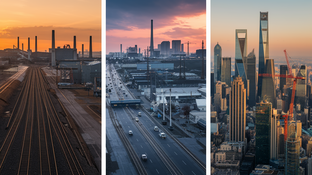
The first big modern supercycle ran roughly 1890 to 1920, driven by the Second Industrial Revolution in the U.S. and Western Europe. Railways expanded across continents. Steel for tracks and bridges, copper for telegraph wires, coal to power steam engines. Factories electrified, cities went vertical with steel-frame construction, agricultural mechanization demanded more land and fertilizer. This was physical infrastructure and the shift from farms to factories, concentrated in a relatively small number of advanced economies modernizing fast.
Post-World War II reconstruction, roughly 1945 to late 1970s, reflected something different. Europe and Japan rebuilt shattered industrial bases, urban centers, transport networks. Energy demand surged as manufacturing returned and car ownership spread. Government-led reconstruction programs and Marshall Plan capital funneled into heavy manufacturing, steel production, basic materials. Unlike the earlier wave, this cycle combined wartime destruction with Cold War development spending and the emergence of consumer economies. Demand was both rebuilding what was lost and creating new consumption patterns—home appliances, suburban housing, highways—that sustained commodity demand for decades.
China’s 2000 to 2011 supercycle introduced a third pattern: emerging-market hyper-growth at unprecedented scale. Between 2000 and 2015, China’s share of global commodity consumption rose from low single digits to dominant positions in steel, copper, coal, cement. Urbanization accelerated. Hundreds of millions moved from rural areas to cities, each new resident requiring housing, appliances, transportation, power infrastructure. Manufacturing capacity expanded to serve global export markets, multiplying demand for industrial metals and energy. Oil climbed from under $20 in 1999 to over $140 in 2008. Copper, iron ore, nickel, coal all posted multi-year runs. This cycle was unique in speed and concentration. One country industrializing faster than entire continents had in prior cycles.
| Cycle | Dates | Key Demand Drivers |
|---|---|---|
| Second Industrial Revolution | ~1890–1920 | Railways, steel mills, electrification, factory buildout in U.S. and Europe |
| Post-War Reconstruction | ~1945–late 1970s | European and Japanese rebuilding, Marshall Plan infrastructure, suburban and consumer expansion |
| China-Led Emerging Markets | ~2000–2011 | Urbanization, manufacturing export capacity, infrastructure at unprecedented scale |
Understanding Industrial Metals and Energy Behavior Within Commodity Supercycles

Industrial metals respond to physical consumption. Copper, aluminum, nickel, zinc go into buildings, power grids, vehicles, machinery. Their demand ties directly to construction activity, manufacturing output, infrastructure investment, making them early-cycle leaders when economies industrialize or rebuild. Energy commodities—oil, natural gas, coal—power those same activities but also serve transportation, heating, electricity generation, creating demand patterns that overlap with but differ from metals. Metals are durable. Once installed, they sit there for decades. Energy gets consumed and must be continuously supplied, making energy markets more sensitive to short-term supply disruptions, geopolitical risk, inventory swings.
Copper and oil serve as bellwethers for different reasons. Copper is essential to construction, power infrastructure, manufacturing. An economy building out housing, factories, or renewable energy needs copper in wiring, motors, transformers, EV charging networks. During China’s 2000s expansion, copper rose roughly fourfold because every new apartment block, factory, power line required incremental metal. Oil reflects economic activity through transportation fuel, petrochemical feedstocks, energy-intensive industries. Its price responds to demand growth but also OPEC production decisions, refining capacity, geopolitical events. Oil surged from under $20 per barrel in 1999 to over $140 in 2008, driven by China’s industrialization and global economic expansion, then collapsed when financial crisis hit and demand fell sharply.
Electrification reshapes metals markets by multiplying the intensity of use per unit of economic output. Electric vehicles require roughly five to ten times more copper than internal combustion vehicles. Wiring, batteries, charging infrastructure, grid upgrades all demand incremental metal. Wind turbines use multiple tons of rare earth elements in generators and magnets. Solar panels require silver, aluminum, specialized alloys. Grid-scale batteries need lithium, cobalt, nickel, graphite. As renewable energy and EV adoption accelerate, demand for these metals rises structurally, independent of traditional GDP growth. This is a policy-driven, secular shift. Governments mandate emissions reductions, subsidize clean energy, ban combustion engines, creating visible, multi-decade demand trajectories that differ from cyclical swings.
Category-specific constraints determine which commodities tighten first. Base metals like copper face declining ore grades. Miners extract lower-quality rock as high-grade deposits deplete, raising production costs and slowing output growth. Lithium and cobalt suffer from geographic concentration. Most lithium comes from hard-rock mines in Australia and brine operations in South America. Most cobalt is mined in the Democratic Republic of Congo, creating geopolitical and ethical supply-chain risks. Nickel production for batteries requires specific chemical grades that only a subset of mines can deliver. Rare earths are geopolitically sensitive because refining capacity is concentrated in China, and building alternative supply chains takes years of investment and regulatory approval.
Metals with the strongest structural tailwinds:
Copper. Essential for electrification, renewable energy, EV infrastructure. Demand projected to grow roughly 65 percent between 2020 and 2030.
Lithium. Battery-grade lithium demand expected to rise 220 percent between 2020 and 2030 as EV adoption accelerates and grid storage expands.
Cobalt. Used in lithium-ion battery cathodes. Demand projected to grow 150 percent between 2020 and 2030, with supply concentrated in politically complex regions.
Nickel. Critical for high-energy-density batteries. Demand anticipated to increase 110 percent between 2020 and 2030, driven by EVs and stationary storage.
Rare earth elements. Indispensable for wind turbine magnets, EV motors, electronics. Supply chains geographically concentrated and politically sensitive.
Battery Metals and Electrification
Lithium, cobalt, nickel, copper face severe supply constraints precisely when demand is accelerating. Lithium carbonate and hydroxide production requires either hard-rock mining followed by chemical processing or evaporation from brine pools, which takes months and requires specific geologic and climatic conditions. New lithium projects take years to permit and ramp. Cobalt supply is dominated by a single country with governance challenges, and ethical sourcing requirements limit how quickly new capacity can scale. Nickel for battery-grade sulfate comes from specific ore types, and converting Class 2 nickel (used in stainless steel) to battery-grade requires additional refining steps. Copper mining has been underinvested globally since the 2016 downturn, and new large-scale copper mines are increasingly rare. These constraints collide with EV sales growth, renewable energy buildouts, grid modernization, creating the potential for sustained deficits and elevated prices.
Supply Constraints, Cost Curves, and Why Supercycles Persist Longer Than Expected

Capital expenditure cycles in mining and energy operate on timelines measured in years, not quarters. A copper mine moves from exploration discovery to first production over seven to twelve years. Geological surveys, drilling, feasibility studies, permitting, environmental assessments, financing, construction, ramp-up. Oil and gas projects face similar or longer timelines for offshore deepwater fields, LNG terminals, pipelines. When commodity prices collapse and stay low—as they did for many materials between 2011 and 2020—producers cut exploration spending, cancel expansion projects, mothball marginal operations, focus on cost reduction and debt paydown. This underinvestment creates the supply deficit that fuels the next cycle, but the lag means prices must stay elevated long enough to justify multi-billion-dollar commitments before new supply even begins construction.
Rising marginal production costs amplify supply constraints. Ore grades decline as miners exhaust shallow, high-grade deposits and move to deeper, lower-grade rock. Extracting the same amount of copper or nickel from lower-grade ore requires more energy, more waste rock removal, more processing chemicals, raising unit costs. Environmental regulations tighten over time. Tailings management, water use, emissions standards, land reclamation, adding compliance expenses and lengthening permitting timelines. Labor costs rise in mining-intensive regions as skilled workers become scarce and safety standards improve. Marginal cost curves shift upward, meaning new supply only becomes economically viable at higher prices, which supports elevated equilibrium price levels even as demand moderates.
The late-cycle surge in new supply typically ends supercycles. After years of high prices, multiple projects reach production simultaneously. Mines that started development during the boom all come online within a narrow window. Capital poured into exploration during the peak discovers new deposits that enter feasibility and construction. Technological improvements or higher prices make previously uneconomical reserves viable, adding incremental supply. This wave of new production often arrives faster than demand can absorb it, especially if economic growth slows, policy changes, or efficiency improvements reduce per-unit consumption. Markets flip from deficit to surplus, inventories build, prices collapse. The 2011 to 2016 commodity downturn followed exactly this pattern. China’s infrastructure spending slowed, new mines ramped globally, broad commodity prices fell 50 to 70 percent from peaks.
Macro Policy, Monetary Cycles, and the U.S. Dollar’s Influence on Commodity Supercycles

Monetary policy shapes commodity prices through real interest rates, inflation expectations, and the opportunity cost of holding physical assets versus financial ones. When central banks cut rates and expand balance sheets—quantitative easing, pandemic-era stimulus—real yields fall and inflation expectations rise, making commodities more attractive. Low or negative real rates reduce the carrying cost of holding non-yielding assets like gold or inventories of oil and copper. Fiscal stimulus that funds infrastructure, defense, energy projects directly increases commodity demand. Tightening cycles that raise real rates and reduce liquidity tend to pressure commodity prices, especially if they slow economic growth and reduce physical consumption.
The U.S. dollar’s strength or weakness directly affects global commodity prices because most commodities are priced in dollars. A weaker dollar makes commodities cheaper in local-currency terms for non-U.S. buyers, stimulating demand and lifting prices. A stronger dollar has the opposite effect. Commodities become more expensive abroad, dampening demand and pressuring prices. Dollar weakness often coincides with periods of U.S. monetary easing, fiscal expansion, or deteriorating confidence in dollar-denominated assets, creating an environment where commodity supercycles flourish. Dollar strength, often driven by Fed tightening or safe-haven demand, tends to cap or reverse commodity rallies, even when physical fundamentals remain tight.
Gold behaves differently from industrial commodities because it responds primarily to monetary dynamics rather than physical consumption growth. Inflation, currency debasement, negative real rates, financial uncertainty drive gold demand. It’s a store of value and hedge against fiat currency risk, not an input to production. During commodity supercycles, gold often benefits from the same inflationary and monetary forces that lift industrial metals and energy, but its drivers are distinct. Copper rises because economies build infrastructure. Gold rises because investors fear inflation or monetary instability. Both can occur simultaneously, but gold can decouple if real rates rise or financial stress eases, even as industrial commodities remain supported by tight physical markets.
Futures Curves, Roll Yield, and Tactical Considerations for Commodity Exposure

Commodity futures trade in term structures that reflect market expectations for supply, demand, storage costs, convenience yield. Backwardation occurs when near-term contracts trade at a premium to deferred contracts, signaling physical tightness. Buyers pay up for immediate delivery because inventory is scarce or demand is urgent. Contango is the opposite. Deferred contracts cost more than spot, reflecting ample supply, high storage costs, weak near-term demand. For investors holding futures-based commodity exposure, the shape of the curve determines roll yield—the gain or loss incurred when rolling expiring contracts into the next month or quarter.
Backwardation creates positive roll yield because investors sell expensive near-term contracts and buy cheaper deferred ones, capturing the price difference as profit over time. During supercycles, persistent backwardation is common. Physical markets tighten, inventories fall, users compete for prompt delivery. This roll yield can add several percentage points annually to total returns, making futures-based ETFs and direct futures positions more attractive. Contango erodes returns. Investors sell low and buy high when rolling, bleeding value even if spot prices remain stable. Deep contango often appears late in cycles or during oversupply, when storage fills and near-term demand is weak.
How roll yield influences commodity ETFs depends on the structure and rebalancing rules.
Futures-based ETFs in backwardation earn positive roll yield, amplifying spot price gains and cushioning spot price declines.
Futures-based ETFs in contango suffer negative roll yield, which can offset or reverse spot price gains and deepen losses during spot declines.
Physically-backed ETFs (gold, silver) avoid roll yield entirely because they hold metal in vaults rather than futures contracts.
Equity-based commodity ETFs track mining or energy stocks, which respond to commodity prices but also to company-specific factors. Leverage, management, costs, introducing different risk-return dynamics than direct commodity exposure.
| Curve Shape | Impact on Futures-Based Exposure |
|---|---|
| Backwardation | Positive roll yield; enhances returns when markets are physically tight; common during supercycles. |
| Contango | Negative roll yield; erodes returns; often signals oversupply or weak near-term demand; typical late-cycle or during gluts. |
Commodity Allocation Vehicles and How to Build Exposure During Supercycles
Mining and energy equities offer leveraged exposure to commodity prices because operating leverage magnifies earnings swings. A 20 percent rise in copper prices can double or triple the free cash flow of a well-run copper miner, driving share prices higher. Equities also pay dividends, provide management and operational optionality, can be held in standard brokerage accounts. The downside is company-specific risk. Operational failures, cost overruns, political expropriation, environmental incidents, poor capital allocation can undermine returns even when the underlying commodity performs. Diversified mining ETFs reduce single-stock risk but still carry sector-wide risks like regulatory changes, labor strikes, broad equity market sentiment.
Commodity futures provide direct price exposure without company-specific noise, making them useful for pure tactical bets or portfolio hedges. Futures require margin accounts, daily mark-to-market, active management of contract rolls. They eliminate dividends and operational risk but introduce roll yield risk and require more hands-on oversight. For investors seeking passive commodity exposure, futures-based ETFs and exchange-traded products bundle futures into tradable securities, handling rolls and margin internally. These products track commodity indices or single commodities, offering liquidity and simplicity at the cost of management fees and potential roll yield drag in contango markets.
Physical commodity exposure—owning gold bars, silver coins, allocated metal in vaults—removes counterparty risk, roll yield, futures curve dynamics. Physical holdings are straightforward. The investor owns the metal, stores it securely, sells when ready. Storage and insurance costs act as a carrying cost, similar to a negative yield. Physical exposure works best for precious metals where storage is practical. It’s impractical for oil, natural gas, bulk industrial metals. Physically-backed ETFs (gold and silver funds holding bullion) bridge the gap, offering the benefits of physical ownership with the liquidity and custody convenience of an exchange-traded security.
Commodity-linked bonds and structured products provide exposure with defined risk-return profiles. Principal protection, capped upside, leveraged participation. These instruments suit investors who want commodity exposure within fixed-income allocations or need downside protection. They introduce credit risk (the issuer’s solvency), complexity, often unfavorable fee structures, so they require careful due diligence.
Pros and cons of each vehicle:
Mining and energy equities. High leverage to commodity prices, dividend potential, company-specific risks, equity market correlation.
Commodity futures. Direct price exposure, no company risk, requires active management, roll yield risk, margin and liquidity requirements.
Futures-based ETFs. Passive and liquid, roll yield drag in contango, tracking error, management fees, no dividends.
Physical commodities or physically-backed ETFs. Eliminates roll and counterparty risk, storage and insurance costs, limited to precious metals practically.
Commodity-linked structured products. Defined risk-return, downside protection options, credit risk, complexity, fees can erode returns.
Portfolio Construction Frameworks for Navigating Commodity Supercycles

Strategic commodity allocation begins by determining the long-term role of commodities in a portfolio. Inflation hedge, diversification from equities and bonds, thematic bet on structural demand shifts. A baseline allocation of 5 to 15 percent in commodity-linked assets provides meaningful diversification without overwhelming the portfolio. Within that envelope, diversify across commodity types—metals, energy, agriculture—and across exposure vehicles—equities, futures, physical. This reduces single-commodity risk, supply-chain concentration, vehicle-specific risks like roll yield or operational failures. Rebalance periodically to maintain target weights and capture gains when one commodity or vehicle outperforms.
Risk control starts with position sizing and stress testing. Commodities are volatile. 20 to 30 percent annual swings are common, and drawdowns during late-cycle corrections can exceed 50 percent. Size positions so a full reversal in one commodity doesn’t impair the overall portfolio. Use scenario analysis to model how the portfolio performs if oil falls 40 percent, copper doubles, or the dollar strengthens sharply. Stress test geopolitical risks. What happens if a major producing country nationalizes mines, or if trade restrictions cut off critical supply chains? Identify concentrations—too much exposure to a single country, company, commodity—and diversify or hedge accordingly.
Timing commodity exposure requires recognizing where in the capital expenditure and supply cycle the market sits. Early in a supercycle, underinvestment is widespread, sentiment is negative, prices sit near or below marginal production costs. That’s when strategic allocations pay off. Mid-cycle, fundamentals tighten, prices rise, narratives shift positive. Tactical allocations and sector rotation work well. Late-cycle, capital floods into new projects, media coverage peaks, phrases like “new normal” or “paradigm shift” dominate. That’s the signal to reduce exposure, lock in gains, prepare for the supply response. Supercycles include corrections and consolidations. Prices pull back but find support at higher lows, so don’t mistake volatility for the end of the cycle. The cycle ends when oversupply is structural, not when prices dip 15 percent after a strong run.
Six portfolio rules for commodity supercycles:
Size allocations to survive full reversals. Commodities can fall 50 to 70 percent peak to trough. Position so losses are manageable within overall portfolio risk limits.
Rebalance on a defined schedule. Quarterly or semi-annual rebalancing captures gains from outperformers and adds to laggards, enforcing disciplined profit-taking.
Stress test geopolitical and supply-chain concentration. Model scenarios where key producers are cut off, prices spike, or alternative sources flood the market. Adjust allocations if exposure is too concentrated.
Stage entry over time, especially early-cycle. Avoid lump-sum bets. Build positions gradually as underinvestment and negative sentiment confirm the setup.
Avoid concentration in single commodities or vehicles. Diversify across metals, energy, exposure types to reduce idiosyncratic risks and roll yield drag.
Set exit criteria tied to capex and supply indicators. When mining capex surges, new projects proliferate, sentiment turns universally bullish, reduce exposure and move to cash or less cyclical assets.
Final Words
We focused on what moves prices now: sustained demand spikes, supply rigidity, rising marginal costs, and policy shifts, signals that favor producer exposure early and diversified positions later. Short timelines matter; new supply lags and late-cycle entries get punished.
Actionable steps are simple: favor producers early, layer into diversified metals and energy exposure, watch capex and futures curves, and size positions for drawdowns.
If you want a tight playbook on what drives commodity supercycles and how to position a portfolio, follow the levels and watchpoints above. The outlook is constructive if these signals hold.
FAQ
Q: What causes a commodity supercycle and what are the potential drivers of the commodity super cycle?
A: The causes of a commodity supercycle are sustained demand growth meeting chronic supply shortfalls, driven by demand surges, supply rigidity, underinvestment, policy shifts, rising production costs, and supply‑chain or geopolitical pressure.
Q: What are the 7 C’s of commodities?
A: The 7 C’s of commodities are Cycle, Consumption, Capacity, Costs, Currency, Country risk, and Climate/regulation — a checklist for demand phase, demand drivers, supply capacity, unit costs, FX, political risk, and policy shifts.
Q: What are the top 3 commodities to invest in?
A: The top three commodities to invest in are copper (electrification and infrastructure demand), lithium (EV and battery growth), and oil (core energy demand and tight supply dynamics); each benefits from long-term structural demand.