

What if a stock can lose 20% overnight even though its earnings haven’t changed?
Volatility does that by raising the return investors demand, which pushes discount rates up and prices down.
Higher beta names and long-duration businesses feel it worst.
This piece explains how spikes in implied or realized volatility flow into wider equity risk premiums, compressed multiples, and temporary mispricings.
Read on to learn the math, the market signals to watch (VIX, beta, forward earnings), and three practical scenarios for investors.
Core Relationship Between Volatility and Stock Valuations

Market volatility directly rewrites what investors demand in return, and that reshapes stock valuations immediately. When the VIX jumps from 15 to 30, investors suddenly want more compensation for holding risky assets. That shift flows into the equity risk premium (ERP), raises discount rates in valuation models, and lowers present values. Higher required returns mean lower valuations. A company projecting $10 million in annual free cash flow might be worth $150 million at a 9% cost of equity but only $125 million at 11%. The difference? Volatility changed how the market prices risk.
Beta makes it worse. Stocks with beta above 1.0 swing harder than the market, so when volatility rises, their required returns climb faster. A 1.2 beta means the stock typically moves 20% more than the index. During volatile periods, that sensitivity translates into steeper discount rates and sharper valuation drops. The numbers back it up: during the February to March 2020 COVID selloff, the S&P 500 dropped roughly 29% as volatility surged. Forward multiples rebounded about 27% by the end of May 2020 compared to the start of the year, showing how fast sentiment and required returns can reverse once volatility settles. In 2022, Ukraine shocks saw prices fall while earnings stayed relatively stable. Tariff announcements in 2025 drove an approximately 8% decline in forward earnings within weeks.
The channel runs through both intrinsic and market-based valuation methods. Discounted cash flow models immediately pull in higher discount rates when volatility spikes, compressing present values. Market multiples like price to earnings or EV/EBITDA often compress during volatile periods as investors apply wider risk margins. Forward earnings estimates can lag market moves by weeks, creating temporary dislocations where prices fall faster than analysts revise projections. You get a valuation environment where the same fundamentals can be priced 10% to 15% lower simply because uncertainty rose.
Five direct valuation consequences of rising volatility:
- Higher equity risk premium raises discount rates and lowers intrinsic value in DCF models
- Multiple compression reduces P/E and EV/EBITDA ratios applied to current or forward earnings
- Wider bid ask spreads and reduced liquidity increase transaction costs and illiquidity discounts
- Forced selling and margin calls create downward price pressure unrelated to fundamentals
- Delayed earnings revisions cause temporary mispricings as markets move faster than analyst updates
Volatility Metrics Used in Stock Valuation Analysis

Implied volatility is the market’s forward looking expectation of price swings, pulled from options prices. The VIX index tracks 30 day implied volatility for S&P 500 options. When it rises from 12 to 25, the market expects twice the daily price movement. Realized volatility measures actual historical price changes over a trailing period (daily, weekly, or monthly) and feeds into models that assume past behavior predicts future risk. Historical volatility is simply realized volatility observed over a specific lookback window, typically 30, 60, or 252 trading days. Beta captures how sensitive a stock is to overall market moves. A 1.5 beta means the stock has historically moved 50% more than the index, amplifying both gains and losses.
Correct measurement matters because small differences compound into large valuation errors. Apple’s 2022 data showed that using volume weighted average prices (VWAP) instead of closing prices produced a volatility estimate roughly 15% lower: 30.0% versus 35.5%. That 5.5 percentage point gap translates into materially different discount rates and option values. ASC 718 accounting guidance requires point in time price observations because standard valuation models assume today’s closing price is the best single forecast for tomorrow, not an average of intraday levels. Averaging prices introduces artificial autocorrelation and understates the true randomness option pricing models require.
Private company valuations rely on public market volatility as a proxy because private shares rarely trade and lack published prices. Analysts map public metrics like the VIX to private discounts for lack of marketability (DLOMs), adjusting for company specific factors. When public volatility rises, private DLOMs typically expand because the already limited market for private shares becomes even less liquid and more uncertain. The mechanics depend on recognizing that volatility isn’t just a statistic. It’s a market signal of risk that investors price into every valuation method.
Four volatility tools investors monitor:
- VIX index for near term market risk expectations
- Historical realized volatility (30 day, 60 day, 252 day) for trend analysis
- Individual stock beta for systematic risk exposure
- Implied volatility skew in options to detect asymmetric downside fears
How Market Volatility Enters DCF and Discount Rate Calculations
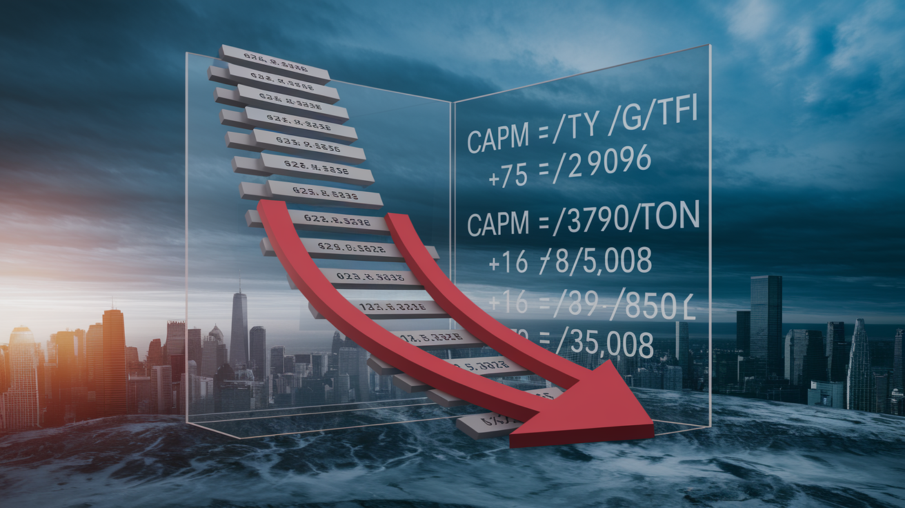
The cost of equity sits at the heart of discounted cash flow models, and volatility changes it directly through the equity risk premium. A standard Capital Asset Pricing Model (CAPM) formula looks like this: cost of equity equals the risk free rate plus beta times the equity risk premium. “Risk free 3% + beta 1.2 × ERP 5% → cost of equity approximately 9%.” When market volatility spikes, the ERP often widens from 5% to 7% or higher as investors demand more return for the same risk exposure. That 2 percentage point ERP increase, multiplied by a 1.2 beta, raises the cost of equity by 2.4 points to around 11.4%. A company with $100 million in perpetual free cash flow is worth $1.11 billion at 9% but only $875 million at 11.4%. A 21% valuation drop driven entirely by the discount rate change.
Beta sensitivity amplifies the effect unevenly across stocks. High beta names (technology growth stocks, cyclicals, small caps) see their required returns rise faster than the market average, while low beta defensive sectors experience smaller increases. A defensive utility with a 0.6 beta might see its cost of equity rise by only 1.2 percentage points under the same ERP expansion, cushioning the valuation impact. Investors often overlook how beta interacts with volatility. The same market shock hits different stocks with very different force depending on their historical co-movement with the index.
Terminal value, which often represents 60% to 80% of total DCF value, compresses sharply when discount rates rise because it discounts distant cash flows at the new higher rate for many years. A company growing at 3% in perpetuity and discounted at 9% has a terminal multiple of roughly 16.7× (1 / [9% − 3%]). Raise the discount rate to 11%, and the multiple falls to 12.5×, a 25% reduction in terminal value. Short term cash flows lose less value because they’re discounted for fewer periods, but the combined effect across all periods still produces double digit valuation declines when volatility driven ERP expansions persist for quarters rather than weeks. The CFO Survey for Q3 2025 identified tariffs, monetary policy, inflation, and skilled labor availability as top concerns, all of which feed uncertainty into discount rate assumptions and widen the range of plausible ERP estimates.
| Input | Volatility Effect |
|---|---|
| Equity Risk Premium | Widens by 1 to 3 percentage points during sustained volatility spikes; directly raises cost of equity and discount rate |
| Beta | Amplifies ERP changes; high beta stocks see larger discount rate increases and steeper valuation declines |
| Risk Free Rate Volatility | Bond market swings change the baseline; rising yields lift discount rates independently of ERP; falling yields can partially offset ERP expansion |
| Terminal Value | Compresses sharply because perpetuity formula is highly sensitive to small discount rate changes; often responsible for majority of total valuation decline |
Market Volatility and Valuation Multiples (P/E, EV/EBITDA, Forward Multiples)

Valuation multiples compress during volatile periods even when underlying earnings remain stable, because the denominator (price) falls faster than analysts revise the numerator. During the COVID selloff from February 20 to March 19, 2020, the S&P 500 dropped approximately 29% while forward earnings estimates lagged behind market sentiment. Analysts didn’t immediately cut their 12 month projections to match the speed of the price decline, so price to forward earnings multiples contracted sharply in real time. By the end of May 2020, the forward multiple had rebounded to roughly 27% above the start of the year, illustrating how multiples can overshoot in both directions when sentiment moves faster than fundamental revisions. Ukraine shocks in 2022 produced a different pattern: prices fell but earnings remained relatively stable through the year, keeping multiples and prices more closely aligned than in the pandemic episode.
Forward earnings themselves introduce timing complexity. Management forecasts and analyst consensus estimates look 12 months ahead, but they update on a lagged schedule (quarterly earnings calls, monthly broker revisions, and periodic resets). When a tariff announcement or central bank surprise hits, markets reprice immediately while earnings estimates take weeks to catch up. The gap creates a window where multiples appear to collapse, not because investors are willing to pay less per dollar of earnings in a steady state, but because the earnings figure in the denominator hasn’t yet reflected the new reality. During the 2025 tariff episode, forward earnings had declined about 8% by the time of writing, but much of that revision came after an initial market selloff. Investors who relied on stale forward EPS data in early April would have seen multiples that looked artificially low, only to normalize as analysts published updated estimates in late April and May.
EV/EBITDA multiples behave similarly but with sector specific nuances. Capital intensive industries (energy, industrials, real estate) often see EBITDA hold up better than net income during volatility because depreciation and interest expenses are excluded, making the EV/EBITDA ratio more stable than P/E in the short run. Technology and consumer discretionary sectors, where operating leverage is high, can experience sharp EBITDA swings that amplify multiple compression. The result is that identical volatility shocks produce different multiple movements depending on the sector’s earnings sensitivity and the market’s view of cyclical versus structural risk.
Five drivers of multiple compression during volatility:
- Earnings revisions lag market price moves by days to weeks, creating temporary multiple dislocations
- Rising discount rates reduce the present value investors assign to each dollar of forward earnings
- Uncertainty about the path of future earnings makes investors demand a risk buffer, lowering the multiple they’re willing to pay
- Forced selling and liquidity concerns push prices down independently of earnings, mechanically compressing multiples
- Sentiment shifts cause investors to re-rate entire sectors or markets lower, applying wider multiples to the same fundamentals
Behavioral Responses to Volatility That Influence Stock Valuations

Panic selling often dominates the first days of a volatility spike, as retail and institutional investors rush to cut exposure before losses deepen. That rush isn’t necessarily irrational. Margin calls, risk management rules, and portfolio constraints can force sales even when an investor believes the long term value hasn’t changed. The result is price pressure that has little to do with fundamentals and everything to do with the structure of the market. Prices fall faster than analysts revise earnings, creating a temporary gap where valuations appear disconnected from intrinsic value. Once the forced selling subsides, prices can rebound sharply even if the fundamental outlook remains murky, as was observed in late May 2020 when forward multiples recovered before economic clarity returned.
Herding amplifies the cycle. When volatility rises, investors look to others for signals about what to do next. If a few large funds start selling, others follow to avoid being the last one holding a falling asset. The feedback loop accelerates price declines beyond what any single rational actor would choose in isolation. Loss aversion (the psychological tendency to feel losses more intensely than equivalent gains) makes investors overweight recent negative outcomes and underweight long term averages. A 10% drop feels worse than a 10% gain feels good, so after a sharp selloff, investors demand higher risk premiums and lower valuations even if objective probabilities haven’t changed much.
Delayed fundamental adjustment creates opportunities and traps. Markets frequently move first and ask questions later. By the time analysts publish revised earnings models, the price has already repriced the new risk. Investors who wait for analyst confirmation often miss the initial move, while those who act on price signals alone can be caught in a sentiment driven swing that reverses within days. The behavioral pattern repeats: fear drives an overshoot to the downside, optimism (or exhaustion of sellers) drives a snapback, and the eventual equilibrium settles somewhere between the panic low and the pre-shock high. Understanding that cycle doesn’t eliminate the risk, but it explains why valuations can vary 15% to 25% over a span of weeks without corresponding changes in long term cash flow expectations.
Liquidity, Market Depth, and Their Valuation Effects During Volatility

Bid ask spreads widen during volatile periods because market makers and liquidity providers demand more compensation for the risk of holding inventory in a fast moving market. A stock that normally trades with a 5 cent spread might see that gap expand to 20 cents or more when volatility doubles. For large institutional orders, the effective cost of trading rises sharply. Executing a $50 million block might require accepting prices 1% to 2% below the last quote simply to find enough buyers. That transaction cost feeds directly into valuation: if selling is expensive, the asset is worth less in the hands of someone who might need to exit quickly.
Private company valuations face even sharper liquidity effects because there’s no continuous market and transactions can take months to complete. Discounts for lack of marketability (DLOMs) measure how much less a private interest is worth compared to an otherwise identical publicly traded share. Empirical studies of restricted stock and pre-IPO transactions commonly indicate DLOMs in the 30% to 50% range under normal conditions. When public market volatility rises, those discounts typically expand because the already limited pool of private buyers becomes more risk averse and the expected time to exit lengthens. Analysts often use the VIX as a proxy for overall market risk and adjust private DLOMs upward when the VIX crosses thresholds like 20 or 30. For more on how market volatility may affect valuation discounts for lack of marketability, including the interaction with company specific factors, see detailed guidance on adjusting DLOMs during periods of heightened uncertainty.
Market depth (the volume of buy and sell orders at prices near the current quote) shrinks when volatility spikes, because participants pull limit orders and wait for clearer signals. Thin markets amplify price swings: a modest sell order that would barely move the price in calm conditions can push it down several percent when depth is low. The effect compounds across asset classes. When equity volatility rises, bond and currency markets often experience simultaneous liquidity contractions, reducing diversification benefits and forcing investors to accept worse execution across their entire portfolio.
Four liquidity driven valuation effects during volatility:
- Wider bid ask spreads raise transaction costs and reduce net realizable value for assets that must be sold quickly
- Reduced market depth means modest order flows move prices more, increasing execution risk and lowering fair value estimates
- Private company DLOMs expand by several percentage points as public market volatility reduces buyer appetite and lengthens expected holding periods
- Forced liquidations during margin calls or redemptions create downward price spirals unrelated to changes in intrinsic cash flow expectations
Case Studies: Volatile Market Episodes and Resulting Valuation Shifts

The COVID-19 market break in early 2020 demonstrated how quickly valuations can disconnect from trailing fundamentals. From February 20 to March 19, 2020, the S&P 500 fell approximately 29% as the WHO declared a pandemic and governments imposed lockdowns. Forward earnings estimates didn’t catch up to the price decline until mid-March through late May, creating a window where price to forward earnings multiples looked unusually compressed. By the end of May 2020, the forward multiple had risen roughly 27% compared to the start of the year, driven by a combination of price recovery and downward earnings revisions that finally reflected the new economic reality. The episode illustrated that markets reprice risk instantly while analysts update models on a quarterly schedule, and the gap between the two creates temporary valuation dislocations that can persist for weeks.
Ukraine’s invasion in early 2022 produced a different pattern. Prices fell as geopolitical risk spiked, but corporate earnings remained relatively stable through the year. Energy and defense sectors saw sharp moves, but broad market earnings didn’t collapse the way they had during the pandemic. Multiples compressed modestly and stayed compressed, because the shock was more about risk premium and uncertainty than about near term cash flow destruction. The valuation effect was smaller in magnitude (mid single digit percentage declines rather than 20% plus drops) but it lingered longer because the geopolitical overhang didn’t resolve quickly.
Tariff announcements in 2025 combined elements of both earlier episodes. An initial U.S. tariff announcement on April 2, 2025 triggered a selloff as investors worried about supply chain disruption and margin compression. A subsequent U.S. China announcement on May 12, 2025 provided some relief and sparked a rally, but forward earnings estimates had already declined by about 8% by the time of writing. A private company valuation relying on S&P 500 comparables would have been approximately 14% lower on April 10, 2025 than on February 20, 2025, purely due to the shift in public market multiples and discount rates. For insights into private company valuations during market volatility, including how illiquid assets lag public market reactions and the importance of scenario based adjustments, see analysis of divergence between public and private valuation responses.
| Event | Key Price Move | Valuation Effect |
|---|---|---|
| COVID-19 (Feb to Mar 2020) | S&P 500 dropped ~29% in under one month | Forward multiples compressed sharply, then rebounded ~27% by end of May as earnings revisions lagged and prices recovered; demonstrated extreme sentiment driven valuation swings |
| Ukraine Invasion (2022) | S&P 500 declined; sector rotation into energy and defense | Modest multiple compression with stable earnings; risk premium expansion rather than cash flow destruction; valuation impact smaller but more persistent |
| Tariff Announcements (2025) | April 2 selloff; May 12 partial recovery | Forward earnings down ~8%; private valuations ~14% lower on April 10 vs February 20; combined sentiment shock and fundamental revision |
How Market Volatility Affects Private Company Valuation Discounts

Private company valuation discounts widen when public market volatility rises because the already limited marketability of private shares becomes even more constrained. Discounts for lack of marketability (DLOMs) compensate investors for the time, cost, and uncertainty of selling an asset that doesn’t trade on an exchange. Empirical studies of restricted stock transactions (publicly traded shares subject to Rule 144 holding periods) and pre-IPO placements commonly show DLOMs in the 30% to 50% range under normal market conditions. When volatility spikes, those discounts typically expand by several percentage points as potential buyers demand more compensation for locking up capital in an illiquid asset during uncertain times. The VIX serves as a common proxy for overall market risk. Practitioners often adjust DLOMs upward when the VIX crosses 20 or 25, reflecting heightened risk aversion across all asset classes.
The expansion isn’t uniform across all private interests. Company specific factors interact with market volatility to determine the final discount. A private company with strong financial performance, diversified revenue, and a clear path to an exit (sale or IPO within 18 months) will see a smaller DLOM increase than a struggling firm with concentrated customer risk and no near term liquidity event. The interaction creates valuation opportunities and risks: wealthy individuals gifting private interests during volatile periods can lock in larger discounts for estate and gift tax purposes, potentially saving meaningful tax dollars if the discounts are properly documented and defensible. But the same volatility makes it harder to justify aggressive discounts to auditors and the IRS, because examiners scrutinize whether the valuation appropriately customized the empirical data to the subject company’s specific characteristics.
Six DLOM drivers that interact with market volatility:
- Put rights or redemption features reduce DLOMs by providing a defined exit path, partially offsetting market illiquidity
- Pool of potential buyers contracts during volatility as acquirers become more risk averse, raising DLOMs
- Company size and financial performance matter more in volatile markets; underperforming or subscale companies see sharply higher DLOMs
- Block size affects execution risk; large blocks are harder to place when buyers are scarce, increasing DLOMs
- Imminent sale or IPO creates a near term market and lowers DLOMs even if broader market volatility is elevated
- Dividend payments increase desirability by providing cash return during the illiquidity period, reducing DLOMs
Modelling Volatility in Valuation Frameworks (Scenario, Sensitivity, Monte Carlo)

Scenario analysis builds multiple versions of the future (base case, upside case, downside case) and assigns probabilities to each. During volatile markets, analysts widen the range between scenarios and often increase the weight on downside outcomes. A base case might assume 5% revenue growth and stable margins, an upside case 8% growth with modest margin expansion, and a downside case flat revenue with 200 basis point margin compression. Volatility changes both the range (upside might stretch to 10%, downside to −3%) and the probabilities (downside probability might rise from 20% to 35%). The weighted average valuation falls not because any single scenario changed dramatically, but because the distribution shifted toward worse outcomes.
Sensitivity tables map how valuation responds to changes in key inputs, typically revenue growth, EBITDA margin, and discount rate. A common approach tests ±2% to ±5% on revenue growth and ±50 to ±150 basis points on the discount rate, then displays the results in a grid. During calm markets, most of the grid shows valuations clustered within 15% of the base case. In volatile periods, the range expands to 30% or more because small input changes compound through the model. Terminal value, which often dominates total value in DCF models, becomes especially sensitive: a 1 percentage point discount rate increase might reduce terminal value by 15% to 20%, and that effect alone can swing the overall valuation by double digits.
Monte Carlo simulation goes further by running thousands of scenarios, each drawing random inputs from specified probability distributions. Revenue growth might be modeled as a normal distribution with mean 4% and standard deviation 3%, while the discount rate follows a distribution centered on 10% with a 1.5% standard deviation. The model runs 10,000 iterations, calculates a valuation for each, and reports the distribution of outcomes (median, 25th percentile, 75th percentile, probability of falling below a threshold). Volatility enters through wider input distributions: if historical volatility has doubled, the standard deviation of growth and discount rate inputs should widen accordingly. The result is a valuation range rather than a point estimate, giving investors a clearer picture of how much uncertainty surrounds the midpoint.
| Model Tool | What Changes Under Volatility |
|---|---|
| Scenario Analysis | Range between upside and downside cases widens; probability weights shift toward downside; base case often revised lower to reflect elevated risk |
| Sensitivity Tables | Input ranges expand (e.g., discount rate ±100 bps becomes ±200 bps); resulting valuation grid shows larger swings and more values outside ±15% of base case |
| Monte Carlo Simulation | Standard deviations of input distributions increase to match observed market volatility; output distribution widens and often skews lower; probability of downside outcomes rises |
| Terminal Value Assumptions | Growth rates often reduced and discount rates increased, compressing terminal multiples; perpetuity growth assumptions tested across wider ranges to capture uncertainty about long run conditions |
Practical Checklist for Assessing Valuations Under Market Volatility

Reassess discount rates immediately when volatility spikes by 50% or more. Check whether the equity risk premium in your CAPM inputs still reflects current market conditions. A 2 percentage point ERP increase translates into a material discount rate change for any stock with beta above 0.5. Update growth assumptions by testing downside scenarios that reflect potential demand destruction, margin pressure, or supply chain disruption. Revisit liquidity assumptions: if the company or fund holds illiquid assets, model the cost and time required to exit during a stressed market. Review valuation multiples from comparable companies and transactions, but apply them with caution. Multiples observed during calm periods may not be relevant when volatility is elevated. Avoid double counting the same risk across multiple adjustments. If you’ve raised the discount rate to reflect market volatility, don’t also apply an extra illiquidity discount that assumes the same risk. For proper techniques on measuring volatility inputs, including why point in time prices matter and how averaging methods can understate risk, see No Free Lunch: Understanding Volatility, Average Prices, and Valuation.
Seven steps for valuing assets during volatile markets:
- Update equity risk premium to reflect current VIX and credit spread levels; test ERP expansion of 1 to 3 percentage points in sensitivity analysis
- Stress test revenue and margin assumptions with downside cases that model realistic demand shocks or cost pressures
- Widen ranges in scenario and sensitivity models to capture the full distribution of possible outcomes; assign higher probabilities to tail scenarios
- Reassess company specific risks that may interact with market volatility (customer concentration, fixed cost leverage, refinancing needs)
- Adjust private company DLOMs upward when public volatility rises, but customize the adjustment to reflect put rights, buyer pool, and near term exit prospects
- Review timing of cash flows and consider liquidity buffers or hedges if the valuation relies on assets that may need to be sold during a downturn
- Document all volatility related assumptions and adjustments transparently to support audit defense and regulatory scrutiny; avoid mechanical reliance on pre-volatility inputs
Final Words
VIX spiked, discount rates moved up, and multiples compressed — that’s the price action we walked through. Those moves cut market prices faster than earnings often change.
Mechanically, higher volatility lifts the equity risk premium, raises required returns, and shrinks forward multiples. Liquidity and behavioral squeezes amplify the effect, and private DLOMs tend to widen.
Now: watch VIX, forward EPS, bid/ask spreads, and margin-pressure cues. Run sensitivity and scenario tests. That’s how market volatility affects stock valuations in practice — with clear signals you can act calmly and stay prepared.
FAQ
Q: How does market volatility affect stock prices?
A: Market volatility affects stock prices by raising required returns and equity risk premia, compressing multiples, widening spreads, and prompting faster price moves than earnings revisions, which lowers valuations near term.
Q: What is the 3 5 7 rule in stocks?
A: The 3 5 7 rule in stocks is an informal timing guideline whose meanings vary; traders often use it to set short, medium and longer holding or review horizons—3, 5 and 7 periods respectively.
Q: What is Warren Buffett’s 70/30 rule?
A: Warren Buffett’s 70/30 rule is an informal allocation guideline often cited as roughly 70 percent equities and 30 percent bonds; Buffett’s published advice, though, generally favors a heavier long‑term equity tilt.
Q: What does a 20 VIX mean?
A: A 20 VIX means the market prices about 20 percent annualized volatility for the next 30 days, implying roughly a 5.8 percent one‑month expected swing in the S&P 500 and higher near‑term uncertainty.